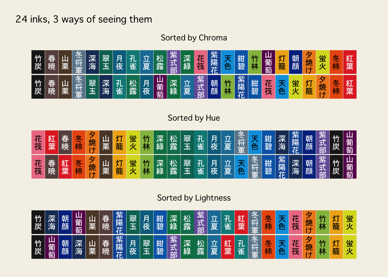
Then I remembered I had also been curious about OKLCH — mostly because I keep seeing it in CSS. So… why not add that too? 😆
Both give me some version of:
lightness
chroma
hue
They aren’t the same colour space, though, so I don’t expect the numbers — or even the ordering — to match perfectly.
Which actually makes this more interesting. What happens when I give the exact same 24 colours two different perceptual coordinate systems?
Same inks, different order
The 24 inks themselves haven’t changed. The hex values are exactly the same.
But when I sort them by hue, chroma, or lightness, HCL and OKLCH don’t always agree on the order.
Some inks stay close to the same neighbours.
Others suddenly swap places.
That makes sense: HCL and OKLCH are different perceptual colour spaces, so their coordinates aren’t expected to line up perfectly. But seeing the difference as an actual row of ink swatches makes it much more tangible than comparing columns of numbers.
In other words:
same colours, different map of colour space. 🎨
And that is exactly what made me want to turn the sorting into something interactive.
Now the colour-space control changes the coordinate system itself, not just the order of the tiles.
That is much more fun.
One important caveat: I shouldn’t interpret the numeric scales of HCL chroma and OKLCH chroma as though they were directly comparable. What interests me here is the resulting relative structure of the 24 colours.
What I learned just getting this far
This is my first time putting Observable JS directly inside a Quarto document, and the biggest adjustment so far is that it doesn’t feel like writing another sequence of notebook cells.
There are a few different things happening:
R prepares the dataset.
Quarto passes it into the page.
Observable handles reactive values and dependencies.
Observable Plot draws the browser-side visualization.
Once that clicked, this started to feel much less mysterious.
And I really like the idea that I can keep doing data preparation in R while using JavaScript only for the parts where browser interaction is actually useful.
Source Code
---title: "Making Iroshizuku Interactive with Observable"description: "Taking my tiny fountain pen ink dataset from R into Observable JS for a first interactive colour visualization."author: "Chi"date: "2026-08-29"categories: - r - observable - javascript - dataviz - colorformat: html: toc: true code-fold: true code-tools: true---```{r}#| label: setup#| include: falselibrary(tidyverse)library(colorspace)library(scales)library(farver)```## One tiny dataset, another rabbit hole 🐇🕳️In the previous post, I turned 24 Pilot Iroshizuku fountain pen inks into a tiny shop using `ggplot2`.But while sorting the inks by colour, I started wondering what it would look like if I could rearrange them interactively.I had also been meaning to try something completely new to me: **Observable JS inside a Quarto document**.So this post is partly an ink experiment and partly me figuring out how R, Observable, and Quarto fit together.The plan is pretty small:> Take the same 24 inks, pass the data from R to Observable, and start moving things around.And while I'm here, I want to play with two perceptual colour representations:* **HCL**, which I used in the previous post* **OKLCH**, which I keep seeing pop up in modern web/CSS colour discussionsLet's see where this goes.## The dataSame 24 inks as before.```{r}#| label: ink-data#| echo: trueiroshizuku_colors <-tibble(ink_name =c("Ajisai", "Asagao", "Konpeki", "Amairo", "Kujaku", "Rikka","Tsukiyo", "Shinkai", "Syoro", "Shinryoku", "Suigyoku", "Takesumi","Fuyusyogun", "Chikurin", "Hotarubi", "Hanaikada", "Murasakishikibu","Yamabudo", "Momiji", "Fuyugaki", "Yuyake", "Toro", "Yamaguri", "Syungyo" ),ink_name_japanese =c("紫陽花", "朝顔", "紺碧", "天色", "孔雀", "立夏","月夜", "深海", "松露", "深緑", "翠玉", "竹炭","冬将軍", "竹林", "蛍火", "花筏", "紫式部","山葡萄", "紅葉", "冬柿", "夕焼け", "灯籠", "山栗", "春暁" ),hex =c("#1255A2", "#04318E", "#0368B4", "#00A0DF", "#028986", "#1A7DA5","#016D8C", "#1C3A65", "#077D5E", "#007E4F", "#037261", "#1E1D1E","#6A869A", "#94BD4E", "#D9DA26", "#ED7E93", "#765FA8", "#660D5B","#E12E2C", "#EA5A10", "#EF881F", "#F0B018", "#5B4532", "#674F4D" ),description =c("Hydrangea","Morning Glory","Deep Cerulean Blue","Sky Blue","Peacock","Early Summer","Moonlit Night","Deep Sea","Dew on Pine Tree","Forest Green","Emerald","Bamboo Charcoal","Winter Commander","Bamboo Forest","Firefly Glow","Floating Cherry Blossoms","Murasaki Shikibu","Wild Grape Vine","Autumn Maple Leaves","Winter Persimmon","Sunset Glow","Lantern Light","Wild Chestnut","Spring Dawn" ))```## Two ways of describing colourIn the last post I used HCL to sort the inks.Then I remembered I had also been curious about **OKLCH** — mostly because I keep seeing it in CSS. So... why not add that too? 😆Both give me some version of:* lightness* chroma* hueThey aren't the same colour space, though, so I don't expect the numbers — or even the ordering — to match perfectly.Which actually makes this more interesting. What happens when I give the exact same 24 colours two different perceptual coordinate systems?## Same inks, different orderThe 24 inks themselves haven't changed. The hex values are exactly the same.But when I sort them by **hue, chroma, or lightness**, HCL and OKLCH don't always agree on the order.Some inks stay close to the same neighbours.Others suddenly swap places.That makes sense: HCL and OKLCH are different perceptual colour spaces, so their coordinates aren't expected to line up perfectly. But seeing the difference as an actual row of ink swatches makes it much more tangible than comparing columns of numbers.In other words:**same colours, different map of colour space.** 🎨And that is exactly what made me want to turn the sorting into something interactive.```{r}#| label: prepare-ojs-data#| echo: true# HCL / polar LUVhcl_coords <-coords(as(hex2RGB(iroshizuku_colors$hex), "polarLUV")) |>as_tibble() |>rename(hcl_h = H,hcl_c = C,hcl_l = L )# OKLCHoklch_coords <- farver::decode_colour( iroshizuku_colors$hex,to ="oklch") |>as_tibble() |>rename(oklch_l = l,oklch_c = c,oklch_h = h )ink_data <- iroshizuku_colors |>bind_cols(hcl_coords, oklch_coords) |>mutate(original_order =row_number() ) |>select( original_order, ink_name, ink_name_japanese, description, hex, hcl_h, hcl_c, hcl_l, oklch_h, oklch_c, oklch_l )ink_data``````{r}#| label: prepare-colour-space-order#| echo: falseplot_data <- ink_data |>pivot_longer(hcl_h:oklch_l) |>group_by(name) |>arrange(value, .by_group =TRUE) |>mutate(x =row_number()) |>ungroup() |>mutate(prop =str_remove(name, "^(hcl_|oklch_)"),y =fct_reorder(name, value, sum, .desc =TRUE),# Japanese vertical writinglabel_vertical =str_split(ink_name_japanese, "", simplify =FALSE) |>map_chr(~paste(.x, collapse ="\n")),# perceptual lightness of each hex colourtext_colour =if_else( farver::decode_colour(hex, to ="lab")[, "l"] <55,"white","black" ) )plot_data <- plot_data |>mutate(prop_label =recode( prop,h ="Sorted by Hue",c ="Sorted by Chroma",l ="Sorted by Lightness" ) )``````{r}#| label: compare-colour-space-order#| echo: true#| fig-cap: "The same 24 inks sorted by hue, chroma, and lightness in HCL and OKLCH."#| fig-align: center#| out-width: "100%"ggplot(plot_data, aes(x = x, y = y)) +geom_tile(aes(fill =I(hex)),width =0.98,height =0.96 ) +geom_text(aes(label = label_vertical,colour =I(text_colour) ),family ="osaka",lineheight =0.85,size =3.5 ) +facet_wrap(~ prop_label,scales ="free",ncol =1 ) +theme_void(base_family ="osaka") +theme(plot.background =element_rect(fill ="#F5F1E8",colour =NA ),panel.background =element_rect(fill ="#F5F1E8",colour =NA ),strip.background =element_blank(),strip.text =element_text(size =10,face ="bold",margin =margin(b =8) ),panel.spacing =unit(1.1, "lines"),plot.title =element_text(size =12,face ="bold",margin =margin(b =12) ),plot.margin =margin(20, 20, 20, 20) ) +labs(title ="24 inks, 3 ways of seeing them" )```Mostly I just want to get this little table out of R and into JavaScript so I can start moving things around in browser!## R, meet Observable 👋This part felt slightly magical the first time it worked.Quarto's `ojs_define()` lets me create something in R and hand it over to Observable running in the browser.So R says: **Here are my 24 inks.**Observable says: **Thanks. Now let me play with them.**```{mermaid}flowchart LR R[R 🐣<br/>prepare data] --> Q[Quarto 📦<br/>hand it over] Q --> O[Observable ✨<br/>play in the browser]```That handoff is basically the whole experiment.R still does the data wrangling I’m comfortable with. Quarto acts as the bridge. Observable takes over once I want the page itself to react.Reference: https://quarto.org/docs/computations/ojs.html```{r}#| label: send-to-ojs#| output: falseojs_define(inks = ink_data)```The R data frame needs one small reshaping step on the Observable side.```{ojs}ink_rows = transpose(inks)```After that, Observable can work with it like ordinary JavaScript data.```{ojs}Inputs.table(ink_rows, { columns: [ "ink_name_japanese", "ink_name", "description", "hex", "hcl_h", "oklch_h" ], header: { ink_name_japanese: "日本語", ink_name: "Ink", description: "Meaning", hex: "Hex", hcl_h: "HCL Hue", oklch_h: "OKLCH Hue" }})```This tiny handoff was one of the things I really wanted to understand from this experiment.**R prepares the data. Observable gets to play with it in the browser.**---## First Observable experiment: rearrange the inksI'm starting with something very simple.Two controls:**Which colour space?**```{ojs}viewof colour_space = Inputs.radio( ["HCL", "OKLCH"], { label: "Colour space", value: "OKLCH" })```And:**What should I sort by?**```{ojs}viewof arrange_by = Inputs.radio( ["Hue", "Chroma", "Lightness"], { label: "Arrange inks by", value: "Hue" })```Because Observable is reactive, changing either input automatically changes anything that depends on it.I'll first map the selected options to the appropriate data column.```{ojs}sort_field = { if (colour_space === "HCL") { if (arrange_by === "Hue") return "hcl_h"; if (arrange_by === "Chroma") return "hcl_c"; return "hcl_l"; } if (arrange_by === "Hue") return "oklch_h"; if (arrange_by === "Chroma") return "oklch_c"; return "oklch_l";}```And then sort.For hue I want low → high around the colour wheel.For chroma and lightness, I find high → low slightly easier to read.```{ojs}sorted_inks = { const rows = [...ink_rows]; if (arrange_by === "Hue") { return rows.sort((a, b) => a[sort_field] - b[sort_field]); } return rows.sort((a, b) => b[sort_field] - a[sort_field]);}```## The interactive paletteFor my first Observable visualization, I'm deliberately keeping the geometry boring.Each ink is just a coloured tile.The interesting part is that its position is reactive.```{ojs}ink_grid = sorted_inks.map((d, i) => ({ ...d, column: i % 6, row: 3 - Math.floor(i / 6)}))``````{ojs}Plot.plot({ width: 850, height: 420, marginTop: 20, marginRight: 20, marginBottom: 20, marginLeft: 20, x: { axis: null, domain: d3.range(6) }, y: { axis: null, domain: d3.range(4) }, marks: [ Plot.cell(ink_grid, { x: "column", y: "row", fill: "hex", inset: 3, tip: true, title: d => { const prefix = colour_space === "HCL" ? "hcl" : "oklch"; return `${d.ink_name_japanese} · ${d.ink_name}${d.description}${d.hex}${colour_space}Hue ${d[`${prefix}_h`].toFixed(1)}°Chroma ${d[`${prefix}_c`].toFixed(2)}Lightness ${d[`${prefix}_l`].toFixed(2)}`; } }), Plot.text(ink_grid, { x: "column", y: "row", text: "ink_name_japanese", fill: "white", fontSize: 18, dy: -5 }), Plot.text(ink_grid, { x: "column", y: "row", text: "ink_name", fill: "white", fontSize: 11, dy: 14 }) ]})```Try changing both controls.Same 24 inks.Same hex colours.Different representation, different ordering.---## Put the inks into colour spaceSorting is one way to use the coordinates.But I can also stop treating the shelf position as meaningful at all and let the colour coordinates determine where each ink goes.First I'll create generic hue and chroma values based on whichever colour space is selected.```{ojs}colour_space_inks = ink_rows.map(d => ({ ...d, display_h: colour_space === "HCL" ? d.hcl_h : d.oklch_h, display_c: colour_space === "HCL" ? d.hcl_c : d.oklch_c, display_l: colour_space === "HCL" ? d.hcl_l : d.oklch_l}))``````{ojs}max_chroma = d3.max(colour_space_inks, d => d.display_c)polar_inks = colour_space_inks.map(d => { const theta = (d.display_h - 90) * Math.PI / 180; // scale chroma to a plotting radius const r = (d.display_c / max_chroma) * 85; return { ...d, theta, radius_value: r, polar_x: r * Math.cos(theta), polar_y: r * Math.sin(theta) };})lightnessExtent = d3.extent(polar_inks, d => d.display_l)lightnessScale = d3.scaleLinear() .domain(lightnessExtent) .range([20, 58])```Now the same plot can switch between HCL and OKLCH.```{ojs}Plot.plot({ width: 850, height: 500, x: { label: `${colour_space} Hue →`, domain: [0, 360] }, y: { label: `↑ ${colour_space} Chroma`, grid: true }, marks: [ Plot.dot(colour_space_inks, { x: "display_h", y: "display_c", fill: "hex", r: 20, stroke: "white", strokeWidth: 1.5, tip: true, title: d => `${d.ink_name_japanese} · ${d.ink_name}${d.description}H ${d.display_h.toFixed(1)}°C ${d.display_c.toFixed(2)}L ${d.display_l.toFixed(2)}` }) ]})``````{ojs}Plot.plot({ width: 700, height: 700, margin: 40, aspectRatio: 1, x: { axis: null }, y: { axis: null }, r: { range: [12,30] }, marks: [ Plot.frame(), // faint reference rings Plot.circle( [20, 40, 60, 80], { x: 0, y: 0, r: d => d, stroke: "#d9d9d9", fill: null } ), // crosshair guides Plot.ruleX([0], {stroke: "#dddddd"}), Plot.ruleY([0], {stroke: "#dddddd"}), // labels for cardinal hue directions Plot.text( [ {x: 0, y: 95, label: "0°"}, {x: 95, y: 0, label: "90°"}, {x: 0, y: -95, label: "180°"}, {x: -95, y: 0, label: "270°"} ], { x: "x", y: "y", text: "label", fontSize: 11, fill: "#777" } ), Plot.dot(polar_inks, { x: "polar_x", y: "polar_y", fill: "hex", stroke: "white", strokeWidth: 1.5, // use lightness for dot size r: d => lightnessScale(d.display_l), //r: 25, tip: true, title: d => `${d.ink_name_japanese} · ${d.ink_name}${d.description}${colour_space}Hue ${d.display_h.toFixed(1)}°Chroma ${d.display_c.toFixed(2)}Lightness ${d.display_l.toFixed(2)}` }) ]})```Now the **colour-space control changes the coordinate system itself**, not just the order of the tiles.That is much more fun.One important caveat: I shouldn't interpret the numeric scales of HCL chroma and OKLCH chroma as though they were directly comparable. What interests me here is the resulting **relative structure** of the 24 colours.## What I learned just getting this farThis is my first time putting Observable JS directly inside a Quarto document, and the biggest adjustment so far is that it doesn't feel like writing another sequence of notebook cells.There are a few different things happening:**R** prepares the dataset.**Quarto** passes it into the page.**Observable** handles reactive values and dependencies.**Observable Plot** draws the browser-side visualization.Once that clicked, this started to feel much less mysterious.And I really like the idea that I can keep doing data preparation in R while using JavaScript only for the parts where browser interaction is actually useful.