Pakcages Used in This Blog Post
library(tidyverse) # Easily Install and Load the 'Tidyverse'
library(cowplot) # Streamlined Plot Theme and Plot Annotations for 'ggplot2'
library(sf) # Simple Features for R
library(patchwork) # The Composer of Plotslibrary(tidyverse) # Easily Install and Load the 'Tidyverse'
library(cowplot) # Streamlined Plot Theme and Plot Annotations for 'ggplot2'
library(sf) # Simple Features for R
library(patchwork) # The Composer of PlotsWhen I was a kid, my dad made a wooden pentomino puzzle which I don’t remember actually solving it (oops!). Many years later, he recreated it with a 3D printer, and while it’s now a plastic version, my puzzle-solving skills haven’t improved much. Whenever I try to put it away, I find myself searching the internet for solutions. So, I thought—why not save some solutions on my blog? BUT, instead of just posting them, I decided to bring pentominos in R to play around.
Pentominoes are geometric puzzles made up of 12 unique shapes, each consisting of exactly five connected squares. The name comes from the Greek root “penta”, meaning five. The well known Domino 🁓 is 2 connected squares!
Each piece is named after the letter it resembles—like F, L, T, and Z. The challenge? Fit these pieces together to cover a rectangular board (or other shapes) without overlaps or gaps.
Here’s a look at the 12 pentomino pieces: 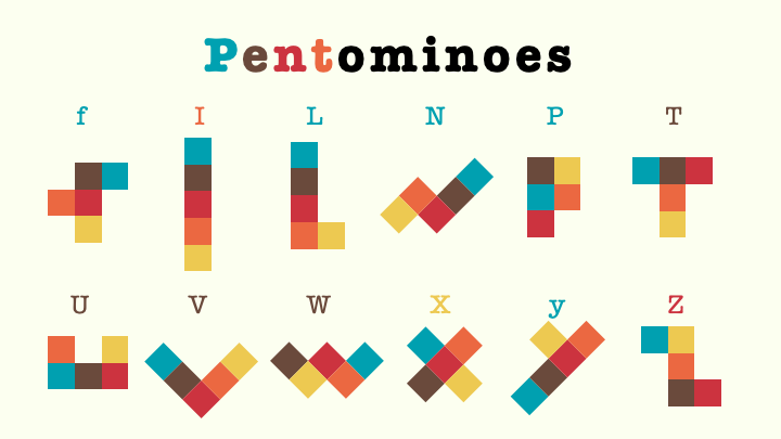
Below is the script to create pentomino_df. Essentially I just recorded coordinates where I should draw a square, so that I can easily draw pentomino pieces with geom_tile function with ggplot2 later!
retro_col5 <- c("#00A0B0", "#6A4A3C", "#CC333F", "#EB6841", "#EDC951")

pentomino_pieces <- list(
  F = list(c(0,0), c(0,1), c(1,1), c(1,2), c(2,1)),
  I = list(c(0,0), c(1,0), c(2,0), c(3,0), c(4,0)),
  L = list(c(0,0), c(1,0), c(2,0), c(3,0), c(3,1)),
  N = list(c(0,0), c(1,0), c(2,0), c(2,1), c(3,1)),
  P = list(c(0,0), c(0,1), c(1,0), c(1,1), c(0,2)),
  T = list(c(0,0), c(0,1), c(0,2), c(1,1), c(2,1)),
  U = list(c(0,0), c(1,0), c(2,0), c(0,1), c(2,1)),
  V = list(c(0,0), c(1,0), c(2,0), c(2,1), c(2,2)),
  W = list(c(0,2), c(1,1), c(1,2), c(2,1), c(2,0)),
  X = list(c(0,1), c(1,1), c(1,0), c(1,2), c(2,1)),
  Y = list(c(0,0), c(1,0), c(2,0), c(3,0), c(2,1)),
  Z = list(c(0,2), c(1,2), c(1,1), c(1,0), c(2,0))
)

# Convert pentomino pieces into a tibble
pentomino_df <- tibble(
  piece = names(pentomino_pieces),
  coords = pentomino_pieces
) %>%
  unnest(coords) %>%  # Expand list of coordinates into rows
  mutate(
    x = map_dbl(coords, ~ .x[1]),  # Extract x coordinate
    y = map_dbl(coords, ~ .x[2])   # Extract y coordinate
  ) %>%
  select(-coords)  # Remove the original list column

# Assign symmetry type to pieces
pentomino_df <- pentomino_df |>
  mutate(rotate_options =
           case_when(piece %in% c("X") ~ 1,
                     piece %in% c("I") ~ 2,
                     piece %in% c("Z") ~ 2,
                     piece %in% c("T","U","V","W") ~ 2,
                     piece %in% c("F","L","N","P","Y") ~ 4),
         flip_options = case_when(piece %in% c("F","L","N","P","Y","Z") ~ 2,
                                  TRUE ~ 1)) |>
  mutate(group_name =
           case_when(piece %in% c("X") ~ "multi-axis",
                     piece %in% c("I") ~ "line-point",
                     piece %in% c("Z") ~ "point",
                     piece %in% c("T","U","V","W") ~ "line",
                     piece %in% c("F","L","N","P","Y") ~ "none"))
What’s the use of dataset, if you don’t visualize them? ;)
### using geom_tile to visualize
pentomino_df |>
  group_by(piece) |>
  ### I just want to give different color to each square
  mutate(idx=row_number(x)) |>
  ggplot(aes(x=x,y=y)) +
  geom_tile(aes(fill=factor(idx)), color="white") +
  geom_text(aes(label=str_c(piece,"\nsym:",group_name)),
            data = . %>%
              group_by(group_name,piece) %>%
              summarise(x=max(x)+0.5, y=max(y+1.5)),
            hjust=1,vjust=1,
            lineheight=0.8, family="Roboto Condensed") +
  facet_wrap(~piece+group_name) +
  scale_fill_manual(values=retro_col5) +
  theme_nothing() +
  coord_fixed()  +
  theme(plot.background=element_rect(fill="#fffff3", color="#fffff300"))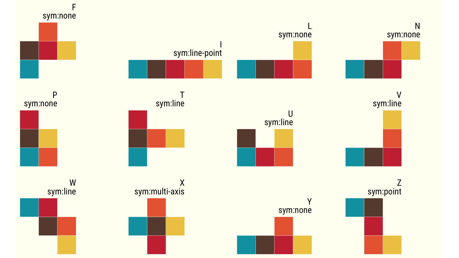
When working with spatial data, converting objects into simple features opens up possibilities for spatial analysis and visualization. The sf package in R provides a user-friendly and standardized way to handle geometric shapes and spatial attributes.
Simple features represent spatial data as geometries (like points, lines, and polygons) alongside their associated attributes. So here’s how I’ve converted data frame with 60 rows into 12 rows with geometry column.
# Function to create a square polygon from a coordinate
# Each coordinate represents the bottom-left corner of a square
create_square <- function(x, y) {
  st_polygon(list(matrix(c(
    x, y,  # Bottom Left
    x + 1, y, #Bottom Right
    x + 1, y + 1, #Top Right
    x, y + 1, #Top Left
    x, y  # Close the polygon by coming back to bottom left
  ), ncol = 2, byrow = TRUE)))
}

# Step-by-step process to convert pentomino data into an sf object
pentomino_sf <- pentomino_df |>
  rowwise() |>
  # For each row, create a square geometry from the x, y coordinate
  mutate(geometry=list(create_square(x,y))) |>
  ungroup() |> # Remove rowwise grouping
  group_by(piece) |>
  # Group all square geometries for each pentomino piece into a single shape
  summarise(geometry=st_union(st_sfc(geometry)),.groups="drop") |>
  # Convert the summarised data into an sf object
  st_sf()

# Write it out as geojson for future use
#pentomino_sf |>
  #st_write(fs::path(here::here(),"posts","pentomino","pentomino_sf.geojson"))

pentomino_sf
Simple feature collection with 12 features and 1 field
Geometry type: POLYGON
Dimension: XY
Bounding box: xmin: 0 ymin: 0 xmax: 5 ymax: 3
CRS: NA
# A tibble: 12 × 2
piece geometry
<chr> <POLYGON>
1 F ((0 0, 0 1, 0 2, 1 2, 1 3, 2 3, 2 2, 3 2, 3 1, 2 1, 1 1, 1 0, 0 0))
2 I ((0 1, 1 1, 2 1, 3 1, 4 1, 5 1, 5 0, 4 0, 3 0, 2 0, 1 0, 0 0, 0 1))
3 L ((0 1, 1 1, 2 1, 3 1, 3 2, 4 2, 4 1, 4 0, 3 0, 2 0, 1 0, 0 0, 0 1))
4 N ((0 1, 1 1, 2 1, 2 2, 3 2, 4 2, 4 1, 3 1, 3 0, 2 0, 1 0, 0 0, 0 1))
5 P ((0 1, 0 2, 0 3, 1 3, 1 2, 2 2, 2 1, 2 0, 1 0, 0 0, 0 1))
6 T ((0 0, 0 1, 0 2, 0 3, 1 3, 1 2, 2 2, 3 2, 3 1, 2 1, 1 1, 1 0, 0 0))
7 U ((0 1, 0 2, 1 2, 1 1, 2 1, 2 2, 3 2, 3 1, 3 0, 2 0, 1 0, 0 0, 0 1))
8 V ((0 1, 1 1, 2 1, 2 2, 2 3, 3 3, 3 2, 3 1, 3 0, 2 0, 1 0, 0 0, 0 1))
9 W ((3 0, 2 0, 2 1, 1 1, 1 2, 0 2, 0 3, 1 3, 2 3, 2 2, 3 2, 3 1, 3 0))
10 X ((2 0, 1 0, 1 1, 0 1, 0 2, 1 2, 1 3, 2 3, 2 2, 3 2, 3 1, 2 1, 2 0))
11 Y ((0 1, 1 1, 2 1, 2 2, 3 2, 3 1, 4 1, 4 0, 3 0, 2 0, 1 0, 0 0, 0 1))
12 Z ((1 1, 1 2, 0 2, 0 3, 1 3, 2 3, 2 2, 2 1, 3 1, 3 0, 2 0, 1 0, 1 1))Now that I’ve transformed my pentomino shapes into sf objects, it’s time to explore the magical world of geometric unary operations! Unary operation is an operation that acts on a single geometric shape to derive a new geometry.
In below, I’m playing around with visualizing my pentomino pieces in layers. Each layer has its own unique touch, an inflated buffer, a deflated outline, as well as the original piece.
Colour of pieces are separated by sysmetry groups. FLNPY pieces are asymetric pieces, while TUVW has line symmetry and so on.
# Quickly Plotting Out with geom_sf
pentomino_sf |>
  left_join(pentomino_df |> select(piece,group_name)) |>
  ggplot() +
  ### puffing it with bigger positive number
  geom_sf(aes(fill=group_name,
              geometry=st_buffer(geometry,dist=1)),
          alpha=0.05, color="snow") +
  ### puffing the geometry by 0.25 to give them little bubble
  geom_sf(aes(fill=group_name,
              geometry=st_buffer(geometry,dist=0.25)),
          alpha=0.3) +
  ### original shape of pentomino pieces
  geom_sf(aes(fill=group_name),color="white") +
  ### deflating just a bit and making it look like stiches
  geom_sf(aes(fill=group_name,
              geometry=st_buffer(geometry,dist=-0.2)),
          color="white",linetype=3) +
  ### deflating closer to the core
  geom_sf(aes(fill=group_name,
              geometry=st_buffer(geometry,dist=-0.45)),
          color="white",linetype=1) +
  facet_wrap(~piece) +
  scale_fill_manual(values=retro_col5) +
  theme_minimal_grid(font_family="Roboto Condensed") +
  labs()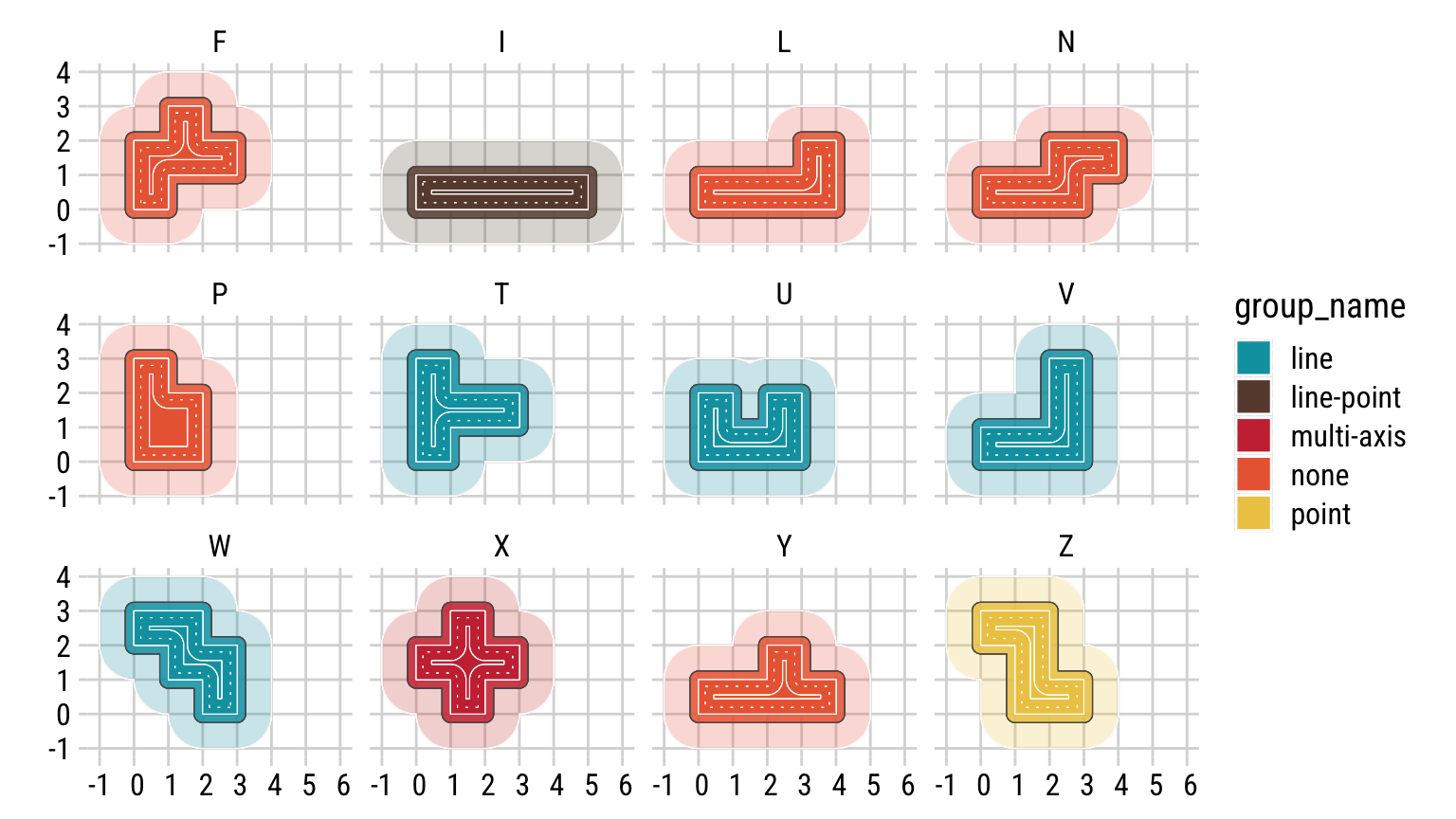
Next up, I just decide to wrap each pentomino in its neatest, smallest rectangle. This is if I were to wrap each pieces in gift wrap. 🎁 The number displayed is the area of rectangle.
These rectangles reveal how tightly we can enclose shapes, which is useful in applications like spatial optimization or determining object orientation in real-life scenario.
# Rotate x degrees around (0,0)
rot <- function(a) {
  a = a*(pi/180)
  matrix(c(cos(a), sin(a), -sin(a), cos(a)), 2, 2)
}

# Visualize pentomino pieces with their minimum rotated rectangles
box_me_up <- function(angle,...) {
  pentomino_sf |>
  mutate(geometry=geometry*rot(angle)) |>
  mutate(mrr_area = st_area(st_minimum_rotated_rectangle(geometry))) |>
  left_join(pentomino_df |> select(piece,group_name)) |>
  ggplot() +
  # Plot rotated rectangles around each shape
  geom_sf(aes(fill=factor(mrr_area),
              geometry=st_minimum_rotated_rectangle(geometry)),
          alpha=0.1,linetype=3, color="black") +
  # Plot original pentomino shapes
  geom_sf(aes(fill=factor(mrr_area)),color="white",alpha=0.9) +
  geom_sf_text(aes(label=mrr_area), family="Roboto Condensed") +
  facet_wrap(~piece) +
  scale_fill_manual(values=c(retro_col5,"#56B870"),guide="none") +
  theme_minimal_grid(font_family="Roboto Condensed") +
  labs(title=str_glue("{angle} degree rotated")) +
  theme(text=element_text(family="Roboto Condensed"),
        axis.text=element_blank()) +
    labs(x="",y="")
}


p1 <- box_me_up(90)
p2 <- box_me_up(180)

p1 + p2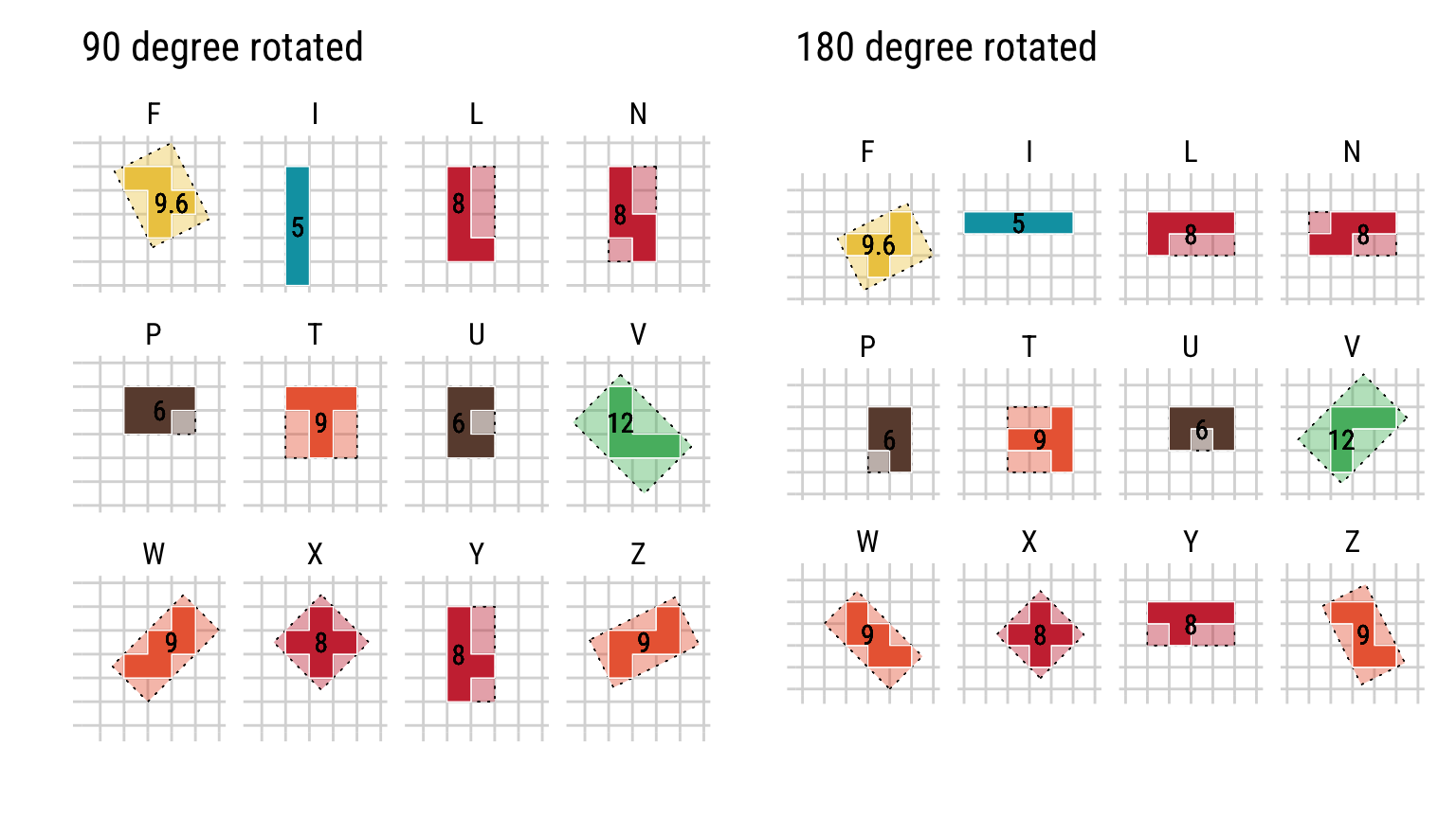
At first, it seemed strange that the F-shape’s rotated rectangle has an area of 9.6, while a simple grid-aligned box could enclose it in an area of 9. The st_minimum_rotated_rectangle function looks for the tightest-fitting rectangle that can enclose the shape. It doesn’t stick to the grid - instead, it tilts the rectangle to snugly fit the shape, even if the result feels counterintuitive? (At least I thought it was counterintuitive…)
For now, I’m wrapping up my geometry experiments (pun intended 🎁).
I’ll dive into how to fit these pieces together to solve the classic pentomino puzzles - No more googling for a solution in next post.