Pentomino Solution & Patchwork

Pentomino Solution as `igraph` object

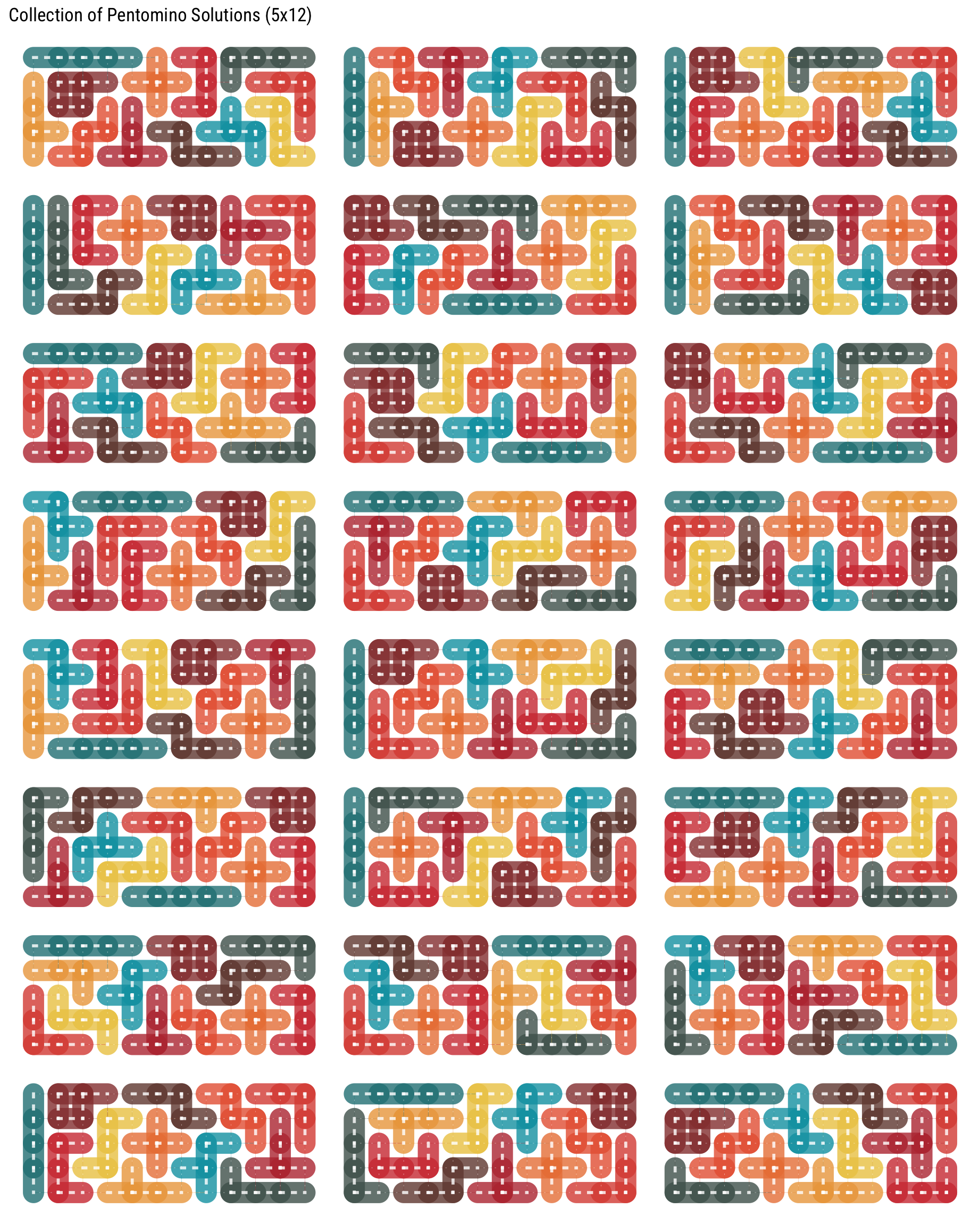
In this post, I’m taking deeper dive into a dataset of Pentomino puzzle solutions using R. This time, I’m switching gears from the sf package, but to explore graph theory concepts with tidygraph and ggraph. Why? Because Pentomino solutions aren’t just puzzles; they’re networks waiting to be uncovered! 🌐

What’s on the menu? 🍴

Data Wrangling with tidyverse
Graphs and graph-based data structures with tidygraph and visualization with ggraph
Arranging Multiple Plots effortlessly with patchwork. The wrap_plots() function function was a lifesaver, sparing me from the monotony of typing plot1 + plot2 + … repeatedly! 🙌

Setups and Pakcages Used

# Load required libraries
library(tidyverse)    # Data wrangling and general utilities
library(ggraph)       # Graph visualization
library(tidygraph)    # Graph data structure (tbl_graph) + graph algorithms
library(ggforce)      # Extra geoms for ggplot2
library(cowplot)      # Additional plotting helpers
library(patchwork)    # Combine multiple ggplots effortlessly!

Original Solution Dataset

I’ve saved solution as csv file from earlier blog posts. So just retriving the dataset. Solution looks like below.

Reading Solution Dataset

### Read solution data frame from Github 
pento_sol <- read_csv("https://raw.githubusercontent.com/chichacha/pentomino/refs/heads/main/pentomino_solution.csv")

sample_n(pento_sol, size=5) |>
  knitr::kable("markdown")

dim	sol_text	row_cnt	col_cnt	sol_idx
5×10	LLLLTTTNNN UUULWTNNFF UPUWWTYFFV PPWWYYYYFV PPIIIIIVVV	5	10	5427
6×10	IIIIIXYYYY VVVFXXXNYW VTFFFXNNWW VTTTFZNWWP UTUZZZNLPP UUUZLLLLPP	6	10	707
5×9	IIIIIFVVV UUPPFFFTV UPPPZZFTV UUNNZLTTT NNNZZLLLL	5	9	1024
8×8d	.FFNNNX. FFNNYXXX IFYYYYXT ILLLLTTT IVVVLWWT IVZZWWPP IVZUWUPP .ZZUUUP.	8	8	133
5×11	LLLLFZZNTTT LXFFFVZNNTY XXXFPVZZNTY UXUPPVVVNYY UUUPPIIIIIY	5	11	2837

Just prepping colors

To make our graphs visually fun, I’m just using retro-inspired color palette and assign unique colors to each Pentomino piece.

Prepping Color Palette

# Just Prepping some color palette
retro <-  c("#00A0B0", "#6A4A3C", "#CC333F", "#EB6841", "#EDC951")
retro12 <- colorRampPalette(retro)(12)
retro13 <- c(retro12,"#ffffff")

#Assigning names to each color allows direct mapping with scale_color_manual() or scale_fill_manual()
piece <- c("F","I","L","N","P","T","U","V","W","X","Y","Z")
names(retro12) <- piece
names(retro13) <- c(piece,".")

retro12 |> enframe() |>
  ggplot(aes(x=name,y=1)) +
  geom_tile(aes(fill=I(value))) +
  geom_text(aes(label=name), color="white",vjust=-0.5) +
  geom_text(aes(label=value), color="white",vjust=1, size=3) +
  theme_nothing()

Converting Solution to (x,y) Positions 📐

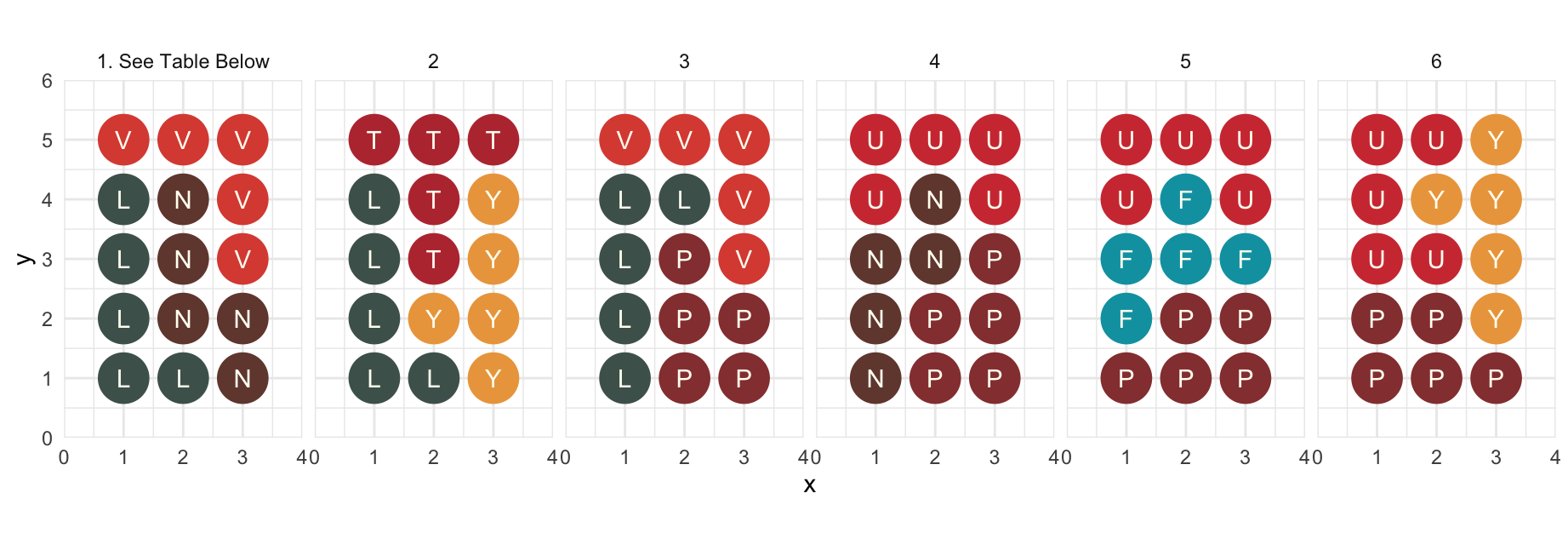
Next, we’ll transform each solution into (x, y) coordinates. This step is crucial for graph creation. I’ve listed a visualization & table of some 3x5 Pentomino solutions, mapped to their (x, y) position.

Converting Solution Texts to Data Frame with Coordinates

### Convert Solution to XY position data frame
pento_sol_df <- pento_sol |>
  mutate(solution_num = row_number()) |>
  mutate(sol_text = str_split(sol_text, " ")) |>
  unnest(sol_text) |>
  group_by(solution_num) |>
  mutate(y = row_number()) |>
  ungroup() |>
  mutate(sol_text = str_split(sol_text, "")) |>
  unnest(sol_text) |>
  group_by(solution_num, y) |>
  mutate(x = row_number()) |>
  ungroup()


# Split the data into chunks programmatically
tables <- pento_sol_df |> 
  filter(dim == "5×3", sol_idx == 1) |>
  select(dim, sol_text, x, y) |>
  group_split(x)

pento_sol_df |> 
  filter(dim == "5×3", sol_idx %in% c(1:6)) |>
  mutate(sol_idx=if_else(sol_idx==1, str_c("1. See Table Below"), as.character(sol_idx))) |>
  ggplot(aes(x=x,y=y)) +
  geom_point(aes(color=sol_text),size=10) +
  geom_text(aes(label=sol_text), color="#fffff3") +
  scale_color_manual(values=retro12, guide="none") +
  theme_minimal() +
  facet_wrap(~sol_idx,ncol=6) +
  coord_fixed() +
  scale_x_continuous(expand=expansion(add=1)) +
  scale_y_continuous(expand=expansion(add=1))

dim	sol_text	x	y
5×3	L	1	1
5×3	L	1	2
5×3	L	1	3
5×3	L	1	4
5×3	V	1	5

dim	sol_text	x	y
5×3	L	2	1
5×3	N	2	2
5×3	N	2	3
5×3	N	2	4
5×3	V	2	5

dim	sol_text	x	y
5×3	N	3	1
5×3	N	3	2
5×3	V	3	3
5×3	V	3	4
5×3	V	3	5

Storing the Solution in Nested Table

Use nest(.by = c(solution_num, dim)) to store each solution’s data in a list column. That way, each row in pento_min corresponds to one puzzle solution, containing the relevant (x, y, sol_text) data in a nested data frame.

Store solution in nested way

pento_min <- pento_sol_df |>
  filter(sol_text != ".") |>  # exclude the "." cells
  select(x, y, sol_text, solution_num, dim) |>
  nest(.by = c(solution_num, dim))

Creating Graphs with tidygraph & ggraph 📈

To visualize the connections between pieces, we’ll use tidygraph to create graph objects and ggraph for plotting.

Function: Data Frame to Graph Conversion

This function converts a solution’s data frame into a graph by identifying adjacent cells.

Convert Data Frame to igraph Object

df_to_graph <- function(data) {
  
  # cross join is expensive, but straightforward: 
  # generate all pairs of cells, then filter to pairs that are adjacent (Manhattan distance = 1).
  tmp <- data |>
    cross_join(data) |>
    filter((abs(x.x - x.y) + abs(y.x - y.y)) == 1) |>
    distinct()
  
  edges <- tmp |>
    transmute(
      from = paste(x.x, y.x, sol_text.x, sep = ","),
      to   = paste(x.y, y.y, sol_text.y, sep = ","),
      w    = if_else(sol_text.x == sol_text.y, 1, 0.1)
    )
  
  # Standardize from/to to avoid duplicate edges in undirected graph
  edges_unique <- edges %>%
    rowwise() %>%
    mutate(
      a = min(from, to),
      b = max(from, to)
    ) %>%
    ungroup() %>%
    distinct(a, b, .keep_all = TRUE) %>%
    select(-a, -b)
  
  graph <- tidygraph::as_tbl_graph(edges_unique, directed = FALSE)
  
  # Add node attributes
  graph <- graph |>
    mutate(
      x     = as.numeric(str_split_i(name, ",", 1)),
      y     = as.numeric(str_split_i(name, ",", 2)),
      piece = str_split_i(name, ",", 3)
    ) |>
    mutate(
      deg   = centrality_degree(weights = w),
      btwn  = centrality_betweenness(weights = w),
      sub_g = centrality_subgraph(),
      idx   = row_number()
    )
  
  return(graph)
}

Function: Graph Visualization

This function plots the graph using ggraph and highlights adjacency within pieces.

Visualizing igraph object with ggraph

plot_graph <- function(g) {
  g |>
    activate("nodes") |>
    mutate(comm = group_louvain(weights = w)) |>
    ggraph(layout = "manual", x = x, y = y) +
    
    # 1) Thicker edges for cells in the same piece
    geom_edge_link(
      lineend = "round", linejoin = "mitre", alpha = 0.8,
      aes(edge_color = .N()$piece[from], edge_width = I(if_else(w == 1, 7, w)))
    ) +
    
    # 2) Another edge layer (white dash) just as decoration
    geom_edge_link(
      lineend = "square", linejoin = "round", alpha = 0.8,
      aes(edge_width = I(w)), color = "#ffffff", linetype = 3
    ) +
    
    coord_fixed() +
    theme_nothing() +
    scale_edge_color_manual(values = retro12) +
    scale_x_continuous(expand = expansion(add = 1)) +
    scale_y_reverse(expand = expansion(add = 1))
  
}

Wrapping It Up with patchwork 🖼️

Finally, let’s use patchwork to combine multiple graphs into a single layout.

Utilizing wrap_plot function

indexes <- c(14369:15378) |> sample(size = 24)

list_of_plots <- indexes %>%
  map(~ {
    pento_min$data[[.x]] %>%
      df_to_graph() %>%
      plot_graph()
  })

wrap_plots(list_of_plots, ncol = 3) +
  plot_annotation(
    title = "Collection of Pentomino Solutions (5x12)",
    theme = theme(text = element_text(family = "Roboto Condensed"))
  ) +
  plot_layout()

Pentomino Solution as igraph object